[Guide] This is a quick tutorial on using object detection based on deep learning to implement a monitoring system. In this tutorial, we use GPU multi-processor to compare the performance of different target detection models on pedestrian detection.
Surveillance is an integral part of security and patrols. In most cases, this work involves observing and discovering things that we do not want to happen for a long time. However, the low probability of emergencies cannot conceal the importance of the ordinary work of monitoring, which is even vital.
It would be great if there were tools that could replace us to "wait and monitor" emergencies. Fortunately, with the advancement of technology in recent years, we have been able to write some scripts to automate the task of monitoring. Before going deeper, we need to consider two issues.
Has the machine reached the level of a human?
Anyone familiar with deep learning knows that the accuracy of image classifiers has surpassed that of humans. Figure 1 shows the classification error rate of humans, traditional computer vision (CV) and deep learning on the ImageNet dataset in recent years.
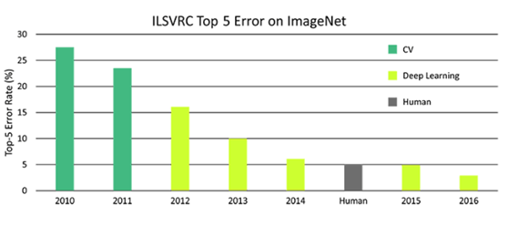
Figure 1 Classification error rate of humans, deep learning and CV on ImageNet
Compared with humans, machines can monitor targets better, and the use of machines for monitoring is more efficient. Its advantages can be summarized as follows:
Repetitive tasks will lead to a decline in human attention, and there is no such annoyance when using machines to monitor. We can focus more on handling emergencies.
When the scope to be monitored is large, a large number of personnel are required, and the field of view of the fixed camera is also very limited. But this problem can be solved by mobile surveillance robots (such as micro drones).
In addition, the same technology can be used for various applications that are not limited by security, such as baby monitors or automated product delivery.
How can we achieve automation?
Before we discuss the complex theories, let's take a look at the normal operation of surveillance. When we watch the live video, we will take action if we find an abnormality. Therefore, our technology should also carefully read each frame of the video to find abnormal things, and determine whether this process requires an alarm.
You may already know that the essence of this process is to locate through target detection, which is different from classification. We need to know the exact location of the target, and there may be multiple targets in a single image. In order to better distinguish, we cite a simple image example as shown in Figure 2.
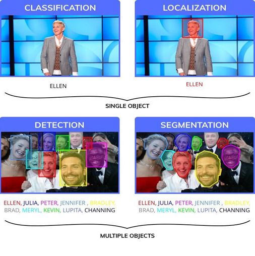
Figure 2 Example diagram of classification, positioning, detection and segmentation
In order to find the exact location, our algorithm should check every part of the image to find the existence of a certain class. Since 2014, continuous iterative research on deep learning has introduced a well-designed neural network that can detect targets in real time. Figure 3 shows the detection performance of the three models of R-CNN, Fast R-CNN and Faster R-CNN in the past two years.

Figure 3 R-CNN, Fast R-CNN and Faster R-CNN performance
There are several deep learning frameworks that use different methods internally to perform the same task. The most popular ones are Faster-RCNN, YOLO and SSD. Figure 4 shows the detection performance of Faster R-CNN, R-FCN and SSD.
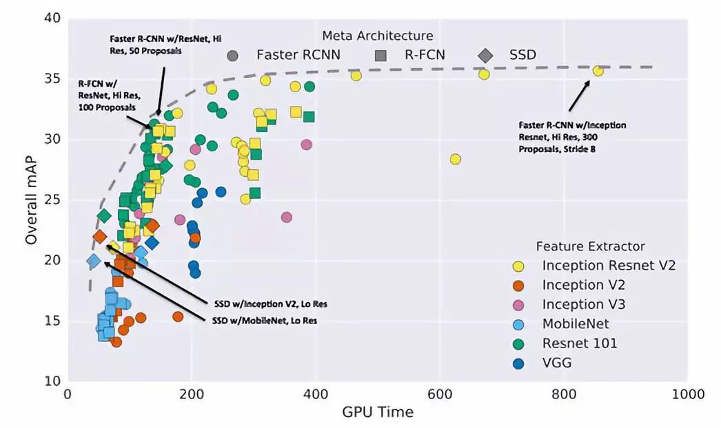
Figure 4 Faster R-CNN, R-FCN and SSD detection performance, the trade-off between speed and accuracy, higher mpA and lower GPU time are the best.
Each model depends on the base classifier, which greatly affects the final accuracy and model size. In addition, the choice of target detector will seriously affect the computational complexity and final accuracy. When selecting a target detection algorithm, the trade-off relationship between speed, accuracy and model size always exists.
With the above learning and understanding, next we will learn how to use target detection to build a simple and effective monitoring system.
Let's start with the discussion of the constraints caused by the nature of the surveillance task.
Limitations of deep learning in monitoring
Before realizing automated monitoring, we need to consider the following factors:
1. Real-time video
In order to observe in a large area, we may need multiple cameras. Moreover, these cameras need to have a place (local or remote location) to store data. Figure 5 shows a typical surveillance camera.
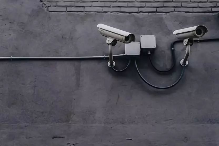
Figure 5 Typical surveillance camera
High-quality video takes up more memory than low-quality video. In addition, the RGB input stream is 3 times larger than the BW input stream. Since we can only store a limited number of input streams, we usually choose to reduce the quality to ensure maximum storage.
Therefore, a scalable surveillance system should be able to resolve low-quality images. At the same time, our deep learning algorithms must also be trained on low-quality images.
2. Processing capacity
Where to process the data obtained from the camera source is another big issue. There are usually two ways to solve this problem.
Centralized server processing
The video stream from the camera is processed frame by frame on a remote server or cluster. This method is powerful and allows us to benefit from high-precision, complex models. But the disadvantage of this method is the delay. In addition, if commercial APIs are not used, the server setup and maintenance costs will be high. Figure 6 shows the memory consumption of the three models as the inference time increases.
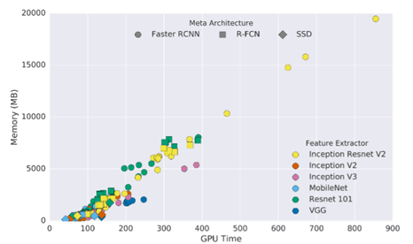
Figure 6 Memory consumption and inference time (milliseconds), most high-performance models will take up a lot of memory
Distributed edge processing
The camera itself is processed in real time by attaching a microcontroller. The advantage is that there is no transmission delay, and feedback can be made faster when an abnormality is found, and it will not be restricted by WiFi or Bluetooth (such as microdrones). The disadvantage is that the microcontroller is not as powerful as the GPU, so only models with lower accuracy can be used. Using the onboard GPU can avoid this problem, but it is too expensive. Figure 7 shows the performance of the target detector FPS.
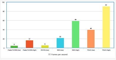
Figure 7 FPS performance of various target detectors
Training monitoring system
In the following content, we will try how to use object detection for pedestrian recognition. Use the TensorFlow target detection API to create a target detection module. We will also briefly explain how to set up the API and train it to perform monitoring tasks. The whole process can be summarized into three stages (the flowchart is shown in Figure 8):
data preparation
Training model
inference
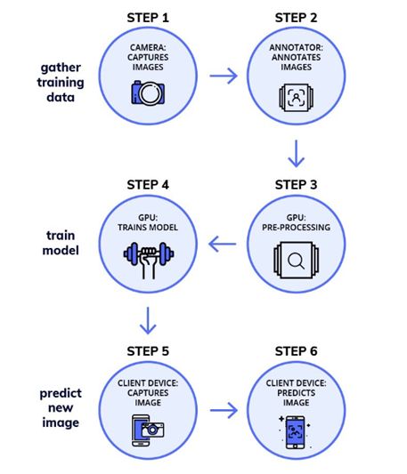
Figure 8 The training workflow of the target detection model
â–ŒPhase 1: Data preparation
Step 1: Get the data set
Surveillance video is the source of the most accurate data set. However, in most cases, it is not easy to obtain such surveillance video. Therefore, we need to train our target detector to recognize targets from ordinary images.
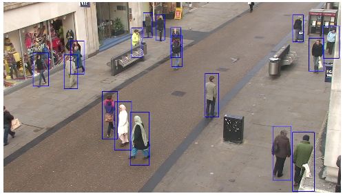
Figure 9 Extracting annotated images from the data set
As mentioned earlier, our image quality may be poor, so the trained model must be adapted to work under such image quality. We add some noise to the images in the dataset (as shown in Figure 9) or try to blur and corrode the images to reduce the quality of the images in the dataset.
In the target detection task, we used the TownCentre dataset. Use the first 3600 frames of the video for training, and the remaining 900 frames for testing.
Step 2: Image annotation
Using a tool like LabelImg for labeling is tedious but also important. We save the marked image as an XML file.
Step 3: Clone the repository
Run the following commands to install the requirements files, compile some Protobuf libraries and set path variables
pipinstall-rrequirements.txt sudoapt-getinstallprotobuf-compilerprotocobject_detection/protos/*.proto--python_out=.exportPYTHONPATH=$PYTHONPATH:`pwd`:`pwd`/slim
Step 4: Prepare the required input
First, we need to give each target a label, and represent each label in the file as label_map.pbtxt as shown below
item{id:1name:'target'}
Next, create a text file containing XML and image file names. For example, if there are img1.jpg, img2.jpg, and img1.xml, img2.xml in the data set, the representation of the trainval.txt file should be as follows:
img1img2
Divide the data set into two folders (images and annotations). Put label_map.pbtx and trainval.txt in the label folder, then create a subfolder named xmls in the label folder, and put all XML files in this subfolder. The directory hierarchy should look like this:
-base_directory|-images|-annotations||-xmls||-label_map.pbtxt||-trainval.txt
Step 5: Create TF record
The API accepts input in the TPRecords file format. Use the creat_tf_record.py file to convert the dataset to TFRecords. We should execute the following commands in the base directory:
pythoncreate_tf_record.py\--data_dir=`pwd`\--output_dir=`pwd`
After the program is executed, we can get train.record and val.record files.
â–ŒPhase 2: Training the model
Step 1: Model selection
As mentioned earlier, speed and accuracy are not at the same time, creating and training a target detector from scratch is very time-consuming. Therefore, the TensorFlow target detection API provides a series of pre-trained models that we can fine-tune according to our own usage. This process is called migration learning, which can greatly improve our training speed.
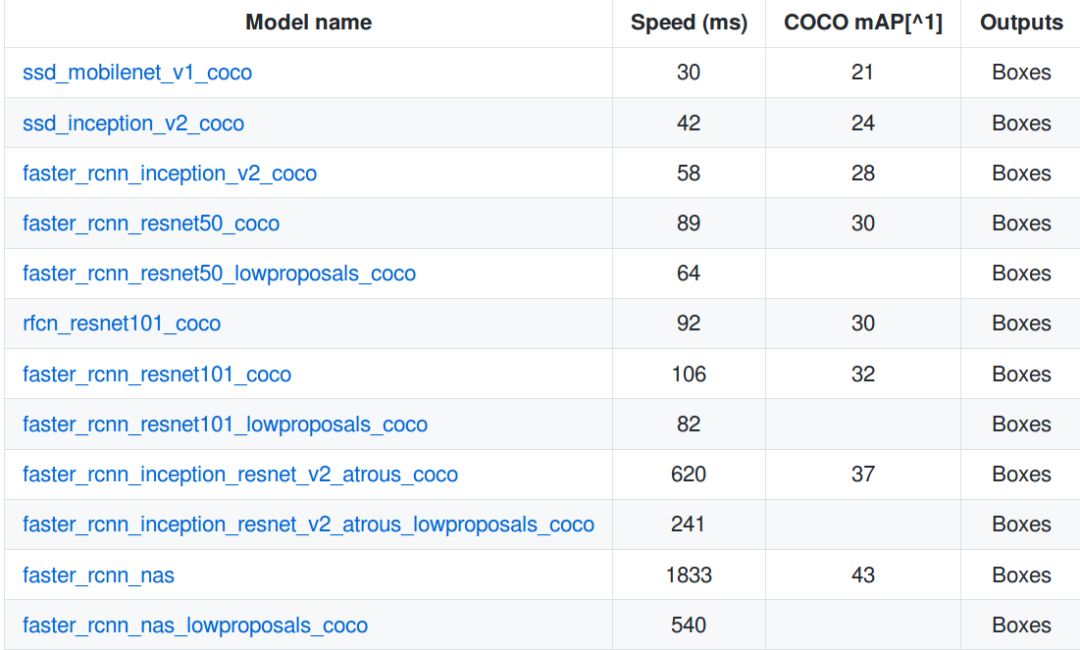
Figure 10 A set of pre-trained models in the MS COCO data set
Download a model from Figure 10, and extract the contents to the base directory. You can get model checkpoints, fixed inference graphs and pipeline.config files.
Step 2: Define the training job
We must define the "training job" in the pipleline.config file and place the file in the base directory. The most important thing in this file is the last few lines-we just need to put the highlighted values ​​in their respective positions.
gradient_clipping_by_norm:10.0fine_tune_checkpoint:"model.ckpt"from_detection_checkpoint:truenum_steps:200000}train_input_reader{label_map_path:"annotations/label_map.pbtxt"tf_record_input_reader{input_path:"train.reader_moving}examplesaver:false label_map_path:"annotations/label_map.pbtxt"shuffle:falsenum_epochs:1num_readers:1tf_record_input_reader{input_path:"val.record"}}
Step 3: Start training
Execute the following command to start the training work. It is recommended to use a computer with a large enough GPU to speed up the training process.
pythonobject_detection/train.py\--logtostderr\--pipeline_config_path=pipeline.config\--train_dir=train
â–ŒPhase 3: Inference
Step 1: Export the training model
Before the model is used, the trained checkpoint file needs to be exported to a fixed inference graph. It is not difficult to implement this process. You only need to execute the following code (replace "xxxxx" with the checkpoint)
pythonobject_detection/export_inference_graph.py\--input_type=image_tensor\--pipeline_config_path=pipeline.config\--trained_checkpoint_prefix=train/model.ckpt-xxxxx\--output_directory=output
After the program is executed, we can get frozen_inference_graph.pb and a bunch of checkpoint files.
Step 2: Use on the video stream
We need to extract each frame from the video source. This can be done using OpenCV's VideoCapture method. The code is as follows:
cap=cv2.VideoCapture()flag=Truewhile(flag):flag,frame=cap.read()##--ObjectDetectionCode--
The data extraction code used in the first stage will automatically create a "test_images" folder for our test set images. Our model can work on the test set by executing the following commands:
pythonobject_detection/inference.py\--input_dir={PATH}\--output_dir={PATH}\--label_map={PATH}\--frozen_graph={PATH}\--num_output_classes=1\--n_jobs=1\ --delay=0
experiment
As mentioned earlier, when selecting a target detection model, speed and accuracy are not compatible. We conducted some experiments on this, measuring the FPS and the accuracy of the number of people detected using three different models. In addition, our experiments are operated under different resource constraints (GPU parallel constraints).
â–ŒSettings
Our experiment selected the following models, which can be found in the Zoo module of the TensorFlow target detection API.
Faster RCNN with ResNet 50
SSD with MobileNet v1
SSD with InceptionNet v2
All models are trained on Google Colab for 10k steps, and the counting accuracy is measured by comparing the closeness between the number of people detected by the model and the actual number of people. Test the inference speed of FPS under the following constraints.
Single GPU
Two GPUs in parallel
Four GPUs in parallel
Eight GPUs in parallel
result
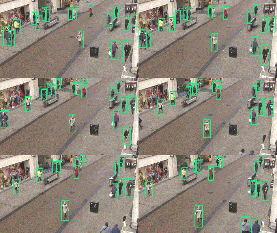
The GIF below is a clip that we output using FasterRCNN on the test set.
â–ŒTraining time
Figure 11 shows the time required to train each model with 10 k steps (unit: hour) (not including the time required for parameter search)
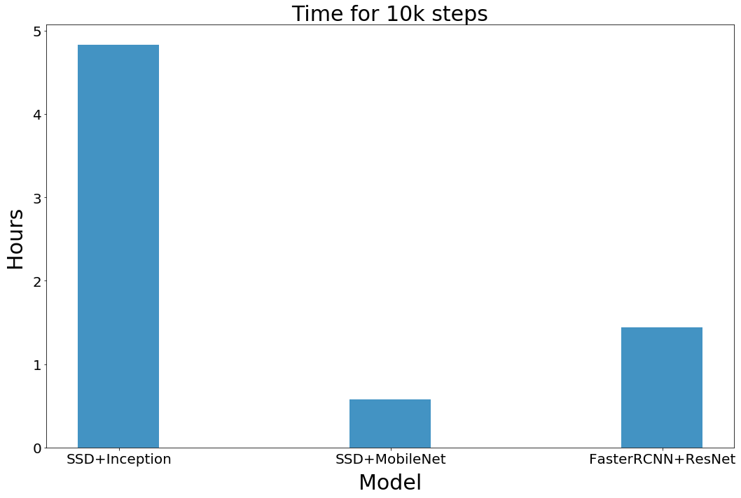
Figure 11 Training time of each model
▌Speed ​​(frames per second)
In the previous experiment, we measured the FPS performance of three models under five different resource constraints. The measurement results are shown in Figure 12:
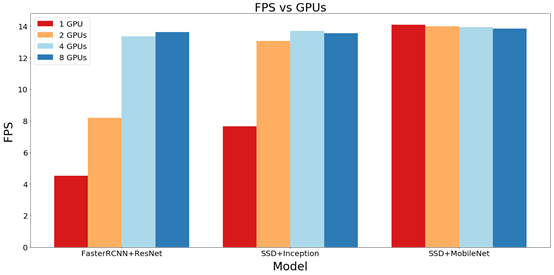
Figure 12 FPS performance under different GPU numbers
When we use a single GPU, the SSD is very fast, easily surpassing the speed of FasterRCNN. But when the number of GPUs increases, FasterRCNN will soon catch up with SSD.
In order to prove our conclusion: the speed of the video processing system cannot be higher than the speed of the image input system, we give priority to reading the image. Figure 13 shows the improvement of FPS with NobileNet + SSD after adding delay. From Figure 13 we can see that when we add delay, FPS increases rapidly.
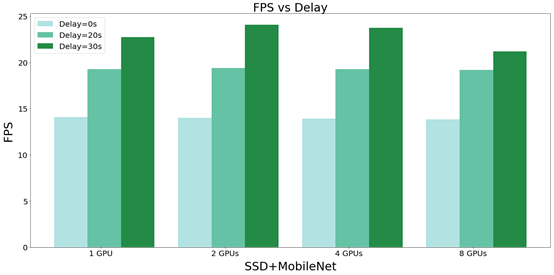
Figure 13 The FPS improvement status of the model after adding different delays
â–ŒCounting accuracy
We define the counting accuracy as the percentage of faces correctly recognized by the target detection system. Figure 14 shows the accuracy of each of our models. It can be seen from Figure 14 that FasterRCNN is the most accurate model, and the performance of MobileNet is better than InceptionNet.
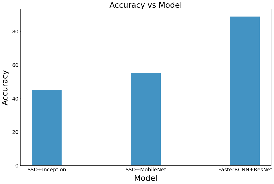
Figure 14 Counting accuracy of each model
Nanonets
Seeing this, I believe everyone has a common feeling-there are too many steps! Yes, if it is such a model, the actual work is heavy and expensive.
For this, a better solution is to use API services that have been deployed on the server. Nanonets provides such an API. They deploy the API on high-quality hardware with GPU so that developers do not have to worry about performance.
The way Nanonets can reduce the work flow is: I convert the existing XML comments into JSON format and provide it to NanonetsAPI. So when you don't want to manually annotate the data set, you can directly request NanonetsAPI to add annotations to the data.
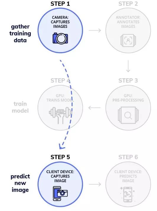
The figure above shows the reduced workflow
The training time of Nanonets took about 2 hours. In terms of training time, Nanonets was the clear winner, and Nanonets also defeated FasterRCNN in terms of accuracy.
FasterRCNNCountAccuracy=88.77%NanonetsCountAccuracy=89.66%
The following shows the performance of the four models in our test data set. Obviously, both SSD models are a bit unstable and have lower accuracy. Although FasterRCNN and Nanonets have higher accuracy, Nanonets has a more stable bounding box.
How reliable is the automatic monitoring?
Deep learning is an amazing tool. But to what extent can we trust our monitoring system and take action automatically? In the following situations, attention needs to be paid when automating the process.
â–ŒSuspicious conclusion
We don't know how deep learning algorithms come to conclusions. Even if the data feed process is perfect, there may be a lot of false success examples. Although guided backpropagation can explain the decision to a certain extent, the research on this aspect still needs our further research.
â–ŒAdversarial attack
Deep learning systems are very fragile, and adversarial attacks are similar to the optical illusion of images. The calculated non-obvious interference will force the deep learning model to misclassify. Using the same principle, researchers have been able to circumvent deep learning-based surveillance systems by using adversarial glasses.
â–ŒFalse alarm
Another question is what should we do if there is a false positive. The severity of the problem depends on the application itself. For example, the false alarms of the border patrol system may be more important than the garden monitoring system.
â–ŒSimilar faces
Appearance is not as unique as fingerprints. Identical twins are the best example. This will cause great interference.
â–ŒLack of diversity in the data set
The quality of deep learning algorithms is very much related to the data set. Google once classified a black man as a gorilla by mistake.
Note: In view of the GDPR and the above reasons, the legality and morality of monitoring automation cannot be ignored. This tutorial is also for the purpose of learning and sharing. The public data set used in the tutorial, so it is the responsibility to ensure its legitimacy during use.
Circuit Test Pen ,Electrical Pen Test,Electrical Test Pen,Test Pencil
YINTE TOOLS (NINGBO) CO., LTD , https://www.yinte-tools.com